


82
MODEL 54eA SECTION 15.0
CALIBRATION - CONTROL
Proportional (Gain) Plus Integral (Reset)
For the automatic elimination of deviation, I (Integral
mode), also referred to as Reset, is used. The propor-
tional function is modified by the addition of automatic
reset. With the reset mode, the controller continues to
change its output until the deviation between measure-
ment and set point is eliminated.
The action of the reset mode depends on the propor-
tional band. The rate at which it changes the controller
output is based on the proportional band size and the
reset adjustment. The reset time is the time required
for the reset mode to repeat the proportional action
once. It is expressed as seconds per repeat,
adjustable from 0-2999 seconds.
The reset mode repeats the proportional action as long
as an offset from the set point exists. Reset action is
cumulative. The longer the offset exists, the more the
output signal is increased.
The controller configured with reset continues to
change until there is no offset. If the offset persists, the
reset action eventually drives the controller output to
its 100% limit - a condition known as "reset windup".
To prevent reset windup, a controller with reset mode
should never be used to control a measured variable
influenced by uncorrectable conditions. Once the con-
troller is "wound up", the deviation must be eliminated
or redirected before the controller can unwind and
resume control of the measured variable. The integral
time can be cleared and the "windup" condition quick-
ly eliminated by manually overriding the analog out-
put using the simulate tests feature (detailed in
Section 5.4).
Control Loop Adjustment and Tuning
There are several methods for tuning PID loops includ-
ing: Ziegler-Nichols frequency response, open loop
step response, closed loop step response, and trial and
error. Described in this section is a form of the open
loop response method called the process reaction
curve method. The reaction times and control charac-
teristics of installed equipment and real processes are
difficult to predict. The process reaction curve method
of tuning works well because it is based on the
response of the installed system. This procedure, out-
lined in the following paragraphs, can be used as a
starting point for the P and I settings. Experience has
shown that PID controllers will do a fair job of control-
ling most processes with many combinations of rea-
sonable control mode settings.
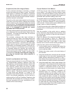
Process Reaction Curve Method
A PID loop can be tuned using the process reaction
curve method. This method involves making a step
change in the chemical feedrate (usually about 50% of
the pump or valve range) and graphing the response of
the Model 54eA controller reading versus time.
The process reaction curve graphically shows the reac-
tion of the process to step change in the input signal.
Figure 14-1 shows an example of a tuning process for
a pH controller. Similar results can be obtained for the
oxygen, ozone, or chlorine controller.
To use this procedure with a Model 54eA controller and
a control valve or metering pump, follow the steps out-
lined below.
Wire the controller to the control valve or metering
pump. Introduce a step change to the process by using
the simulate test function to make the step change in
the output signal.
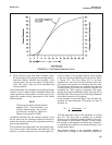
Graph the change in the measured variable (concen-
tration or pH) as shown in Figure 15-1. Observe the
reading on the Model 54eA controller and note values
at intervals timed with a stop watch. A strip chart
recorder can be used for slower reacting processes. To
collect the data, perform the following steps:
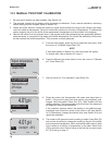
1. Let the system come to a steady state where the
measured variable (pH, concentration or tempera-
ture) is relatively stable.
2. Observe the output current on the main display of
the controller.
3. Using the simulate test, manually set the controller
output signal at the value which represented the
stable process measurement observed in step 1,
then observe the process reading to ensure steady
state conditions (a stable process measurement).
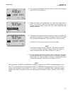
4. Using the simulate test, cause a step change in the
output signal. This change should be large enough
to produce a significant change in the measured
variable in a reasonable amount of time, but not
too large to drive the process out of desired limits.
5. The reaction of the system, when graphed, will
resemble Figure 15-1, showing a change in the
measured variable over the change in time. After a
period of time (the process delay time), the meas-
ured variable will start to increase (or decrease)
rapidly. At some further time the process will begin
to change less rapidly as the process begins to sta-
bilize from the imposed step change. It is important
to collect data for a long enough period of time to
see the process begin to level off to establish a tan-
gent to the process reaction curve.