


USING THE COMBISCOPE INSTRUMENTS 3 - 55
3.9.5 Histogram functions
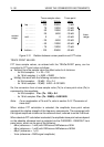
The HISTogram function calculates an amplitude distribution of the incoming trace.
The number of points in the histogram trace is 512. Each point in the histogram
specifies the number of times that a data point of the incoming trace is within a
particular amplitude belt. Since there are 512 histogram points, there are also 512
amplitude belts. The range of the amplitude belts is determined by the selected
peak-to-peak range (SENSe:VOLTage:RANGe:PTPeak) and is expressed by the
following equation:
amplitude belt = peak-to-peak range / 512
Notice that a histogram contains 512 valid data points. The number of points
(TRACe:POINts) of the trace memory location where the histogram is stored, may
exceed this value. In that case the values of the trace positions above 512 have
to be ignored.
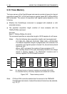
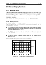
The histogram is displayed on the screen in the area between +3 and -2 divisions
vertically, and between the third and the seventh division horizontally. The
horizontal axis represents the amplitude in volts. The vertical axis represents the
number of occurrences of an amplitude in percents.
PROGRAM EXAMPLE:
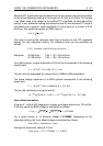
CALL Send(0, 8, "CALCulate:TRANsform:HISTogram:STATe ON", 1)
’
This turns the histogram function on
.
3.9.6 Frequency filtering
The FILTer function performs digital low-pass filtering to suppress undesired
frequency noise. The width of the filter window can be programmed from 3 to 41
points in increments of 2 points. After a
*
RST command, the number of points is 19.
PROGRAM EXAMPLE:
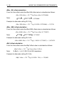
CALL Send(0, 8, "CALCulate:FILTer:FREQuency:POINts 35", 1)
’
35 filter points
CALL Send(0, 8, "CALCulate:FILTer:FREQuency:STATe ON", 1)
’
Filter CALC1 on