


BERT Technical Articles
B-14 GB1400 User Manual
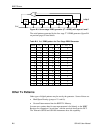
SESs for which the previous two seconds were also SESs. Some BERTs will graph these and
other errors over time to illustrate clumping or mark events.
How long is long enough?
Every time the BERT detects an error, it logs another check mark in the error column and
updates the other various measurements it makes. At what point, however, can you say that the
various measurements give an accurate representation of your system? Consider: With a BER of
10
-15
, a 1 Gb/s system will encounter an error every 11.5 days.
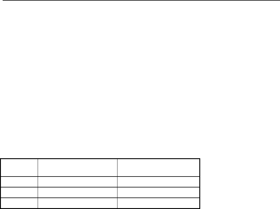
A valid test certainly requires more than a single error to offer statistically relevant results (see
Table 1). Random sampling is just that - random. Your design may have encountered a burst of
errors that won't happen again for another three months (perhaps due to some unusual electrical
interference), but if the sample was not large enough to tell you otherwise, you would consider
the device bad. Also consider the inverse where a bad system appears good.
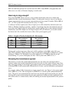
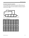
Table 1. Length of Test for Evaluation of 1 Gb/s System
BER
68% confidence
(10 errors)
90% confidence
(100 errors)
10
-9
10 seconds 1.7 minutes
10
-12
2.8 hours 1.2 days
10
-15
116 days 3.17 years
Testing until you have ten errors offers only a 68% confidence in the BER, while 100 errors
offers 90% confidence. Think about how long it would take to obtain 90% confidence in systems
running at 1 Mb/s or 19.2 kilobaud, if you were looking for a 10
-9
BER. So how do you get
around taking 3.17 years to thoroughly test that 1 Gb/s system with a BER of 10
-15
?
Stressing the transmission system
One answer is to stress the system and increase the error rate. Error rates measured while a
system is under stress can be extrapolated to lower error rates for the system with no stress. First,
take a thorough reading of the design's performance under normal operating conditions. Then, by
collecting BERs for the system under different levels of stress, you can determine a performance
curve.
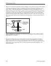
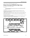
For example, adding 3 dB of attenuation to impair signal levels, (see Figure 1), the system might
show a BER of 5 x 10
-6
. This corresponds to a BER of 10
-10
for the system without attenuation
stress. The goal is not to determine the actual error rate, but the upper bound on the error rate. By
stressing the system and increasing the error rate experienced, testing can take significantly less
time (more errors in a shorter time), while still offering an accurate representation of the system's
quality.