


BERT Technical Articles
GB1400 User Manual B-39
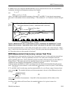
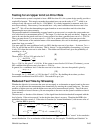
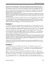
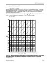
Note that the line through the points in Figure 6 has about the same slope as the dashed lines. This
indicates the noise is about Gaussian. As the slope of the plotted line is closer to that of the dashed lines,
the noise process is closer to Gaussian, and the extrapolation is more reliable. Departure of the slope
from the Gaussian could be due to (a) too few errors measured, leading to inaccurate BER values, (b) the
presence of a non-Gaussian noise mechanism such as error bursts, or (c) significant noise in the system
before the attenuator. (Noise coming into the receiver with the signal is assumed to be less than that
introduced by the first stage in the receiver.)
Whether or not the slope is the expected one, confidence in the extrapolation can always be increased by
taking time to plot out the BER-versus-Attenuation curve once down to very low BER. Thus it may take
a day or so to test the first system, but subsequent systems can then be tested quickly with the stress-and-
extrapolate method.
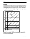
It is important to measure enough errors that the inaccuracy is low and the extrapolation is valid. Because
more than 10,000 errors were measured each time, the inaccuracy of the BER measurement is less than
1% [see Equation (7a)]. This is small enough that the extrapolated results are accurate, even given the
magnification effect of extrapolation. To illustrate the importance of measuring enough errors, we will
look at an example where measuring too few errors leads to uncertain results.
Example 2
A 1.544-Mbit/s system is stressed with 6 dB of electrical attenuation. In a one-second interval 54 errors
are measured––a BER of 54 / 1544000 = 3.5×10
−5
. But with only 54 errors, the inaccuracy is 14% (see
Figure 3 for 68% confidence). Therefore the BER lies between 3.0×10
−5
and 4.0×10
−5
. This uncertainty
is indicated by plotting a bar at 6 dB in Figure 6. Then the electrical attenuation is reduced to 4 dB, and
37 errors are measured in 60 seconds. This is a BER of 37 / (60 × 1544000) = 4×10
−7
. But with 37
errors, the inaccuracy is 16%, and the BER lies between 3.35×10
−7
and 4.65×10
−7
. This is also plotted
as a bar in Figure 6. Straight lines passing through the two bars sweep out the gray region shown and
intersect the BER axis anywhere from 2×10
−15
to 1.5×10
−13
.
The large uncertainty of the extrapolated results in this example is mostly due to the few number of errors
measured. A good rule is to measure at least 1000 errors for each point. Another guideline is to make the
larger attenuation at least 1.5 times the smaller; a greater separation between the two points allows better
extrapolation. Also, use as little attenuation as possible so the extrapolation distance is not so great (this
involves a trade-off with greater test time).
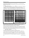
Stressing can also be used to reduce the time required to show that the unstressed BER is below some
specified value. The following example will show how the graph paper provided at the end of the article
can be used in this way.
Example 3
A 1.544-Mbit/s system is to have a BER no more than 10
−9
. This corresponds to an error rate of r =
1544000 × 10
−9
= 0.001544 errors per second. For a confidence C = 95% that the BER of the system is
less than 10
−9
, it must test error-free for T = 3 / r = 1943 seconds, or 32 minutes [see Equation (10)].
This test time can be shortened by using stressing.
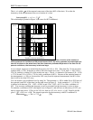
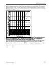
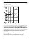
Suppose a system was just on the limit, with an unstressed BER of the specified 10
−9
. Make a plot of
BER versus Attenuation by starting at BER = 10
−9
for Attenuation = 0, and draw a straight line parallel to
the dashed lines, as in Figure 7. We see that 3 dB of electrical attenuation would raise a BER of 10
−9
to
10
−5
, or a stressed error rate of r
s
= 15.44 errors per second. So we stress the system with 3 dB of
attenuation and test it for T
s
= 3 / r
s
= 0.194 seconds. If there are no error in that time, then we have 95%